

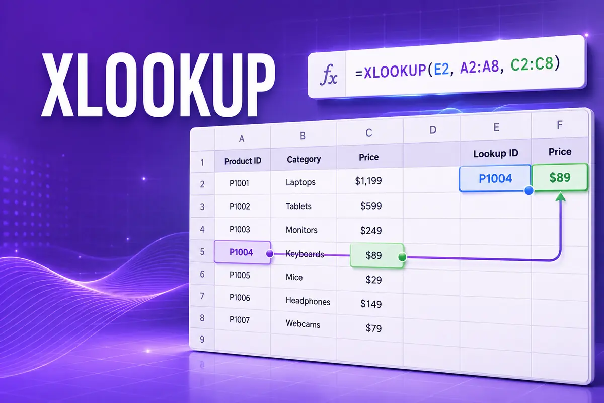
Finding information inside a large spreadsheet can be frustrating, especially when the data contains hundreds or thousands of rows. XLOOKUP makes this task much easier by searching for a value in one range and returning related information from another. It is useful for employee records, product lists, sales reports, student results, stock sheets, and many other business tasks. With a clear formula and flexible search options, the function can replace several older and more complicated lookup methods.
What Is XLOOKUP?
XLOOKUP is a lookup and reference function available in newer versions of Microsoft Excel. It searches a specified row or column for a value and returns the corresponding result from another row or column. Unlike older lookup formulas, it does not require the return data to appear on a particular side of the search column. It also uses an exact match by default, which reduces the risk of returning an unexpected result. Microsoft’s official documentation describes it as a function that searches a range or array and returns the item related to the first match.
XLOOKUP Syntax and Arguments
The basic structure of the formula is:
=XLOOKUP(lookup_value, lookup_array, return_array, [if_not_found], [match_mode], [search_mode])The first three arguments are required, while the final three are optional. The lookup_value is the information you want to find. The lookup_array is the row or column where Excel should search. The return_array contains the answer you want to retrieve. The optional arguments control missing-value messages, matching behavior, and the direction or method used during the search.
Understanding the Required Arguments
The lookup_value may be text, a number, a date, a logical value, or a cell reference. The lookup_array must be the range containing that value, while the return_array must contain the related results. The lookup and return ranges should have compatible dimensions. If one range covers ten vertical cells, for example, the other should normally cover ten vertical cells as well. Mismatched ranges may cause Excel to return an error instead of the expected answer.
A Basic XLOOKUP Example
Imagine that column A contains employee identification numbers and column B contains employee names. If cell E2 contains the identification number you want to find, the following formula can return the employee’s name:
=XLOOKUP(E2,A2:A100,B2:B100)Excel searches cells A2 through A100 for the value entered in E2. Once it finds the matching identification number, it returns the name from the same position in column B. This arrangement is easy to understand because the search range and result range are entered separately.
Why XLOOKUP Is Better Than Older Methods
XLOOKUP solves several limitations associated with traditional lookup formulas. It can search from left to right, right to left, top to bottom, or bottom to top. It does not rely on a fixed column index number, so inserting a new column is less likely to break the formula. It also performs an exact search unless another match mode is selected. These features make spreadsheets easier to maintain, particularly when several people regularly edit or reorganize the same workbook.
XLOOKUP vs. VLOOKUP
VLOOKUP searches the first column of a selected table and normally returns information from a column located to its right. It also requires the user to enter a column index number. If the table structure changes, that number may point to the wrong column. The newer function separates the search range from the result range, allowing data to be returned from either direction. Microsoft also identifies it as an improved alternative that works in any direction and returns exact matches by default.
Creating a Custom “Not Found” Message
A missing lookup value normally produces a #N/A error. Although the error is technically correct, it may confuse people who only need to read the report. The optional if_not_found argument can replace it with a clearer message:
=XLOOKUP(E2,A2:A100,B2:B100,"Employee not found")If the identification number in E2 does not appear in the search range, Excel displays “Employee not found.” A blank string, written as "", can also be used when the result cell should remain visually empty.
Using Exact and Approximate Matches
The optional match_mode argument controls how the formula handles matches. A value of 0 requests an exact match and is the default setting. A value of -1 returns an exact match or the next smaller item, while 1 returns an exact match or the next larger item. A value of 2 enables wildcard matching. Approximate modes are helpful for tax bands, commission levels, shipping charges, grading scales, and other situations where values fall within ranges.
Finding a Price from a Pricing Band
Suppose column A contains minimum order quantities and column B contains the price available at each level. If the quantities are arranged from smallest to largest, the following formula can return the price for the order quantity in E2:
=XLOOKUP(E2,A2:A10,B2:B10,"No price",-1)The -1 match mode asks Excel to find an exact match or the next smaller value. Therefore, an order of 75 units could use the price assigned to the 50-unit band when no separate 75-unit level exists.
Using Wildcards in a Search
Wildcard matching is useful when the complete text is unavailable. An asterisk represents any number of characters, while a question mark represents one character. To find a customer name containing the text entered in E2, you could use:
=XLOOKUP("*"&E2&"*",A2:A100,B2:B100,"No match",2)The final argument used here is the wildcard match mode. This formula could match “Green Valley Foods” when E2 contains only “Valley.” However, it returns the first suitable result, so wildcard searches should be used carefully when similar records exist.
Searching from the Bottom of a List
By default, Excel begins at the first item and returns the first matching result. The optional search_mode can reverse that behavior. A value of -1 searches from the last item toward the first:
=XLOOKUP(E2,A2:A100,C2:C100,"No record",0,-1)This technique is useful for transaction logs, order histories, attendance sheets, or status records. If the same customer number appears several times, searching from the bottom can return the most recently entered record, provided the list is arranged in chronological order.
Returning Multiple Columns
The return range does not have to contain only one column. In versions of Excel that support dynamic arrays, a formula can return several related fields at once:
=XLOOKUP(E2,A2:A100,B2:D100,"No record")If columns B through D contain a product name, price, and stock quantity, Excel can place all three results across neighboring cells. The surrounding cells must be empty, or the formula may produce a #SPILL! error because there is no space for the complete result.
Performing a Horizontal Search
Lookup data is sometimes arranged across rows rather than down columns. The function can handle this layout without requiring a separate horizontal formula. For example:
=XLOOKUP(B5,B1:M1,B2:M2,"Month not found")This formula searches the month headings in B1:M1 and returns the related value from B2:M2. Horizontal searches can be useful in monthly budgets, yearly forecasts, performance dashboards, and reports where time periods are displayed from left to right.
Creating a Two-Way Lookup
A two-way search finds a result by matching both a row label and a column heading. This can be achieved by placing one lookup formula inside another:
=XLOOKUP(H2,A2:A20,XLOOKUP(H3,B1:F1,B2:F20))In this example, H2 may contain a product name, while H3 contains a month. The inner formula identifies the correct month column, and the outer formula identifies the correct product row. The final result appears where those two selections meet.
Looking Up Data from Another Worksheet
The search and return ranges can be located on another worksheet. If a sheet named Products stores item codes in column A and prices in column D, a formula on a different sheet might be:
=XLOOKUP(A2,Products!A:A,Products!D:D,"Code not found")Using full-column references is convenient, but limiting ranges to the actual data area may improve performance in large workbooks. Structured table references are another good option because they expand automatically when new records are added.
Common Reasons a Formula Fails
A lookup may fail because the requested value does not exist, one entry contains extra spaces, numbers are stored as text, or the search and result ranges have different sizes. Text is generally not case-sensitive, so differences in capital letters are not normally the cause. Hidden spaces are more troublesome. The TRIM function can remove unnecessary spaces, while VALUE or -- can help convert numeric text into real numbers when appropriate.
Understanding Common Excel Errors
The #N/A error usually means no matching item was found. A #VALUE! error may point to incompatible ranges or another invalid argument. A #SPILL! error appears when a multi-column result cannot expand because nearby cells contain data. A #NAME? error may indicate that the Excel version does not recognize the function or that its name was typed incorrectly. Checking the lookup value, range sizes, data types, and surrounding cells will solve many of these problems.
Compatibility with Excel Versions
This feature is available in current editions such as Microsoft 365, Excel 2024, and Excel 2021, including supported Mac versions. Older perpetual releases may not recognize formulas that use it. A workbook shared with someone using an unsupported version may display #NAME?. Before replacing older lookup formulas across an organization, confirm which Excel editions are installed on the computers that will open and edit the file.
Tips for Building Reliable Lookup Formulas
Use fixed references such as $A$2:$A$100 when copying formulas to other cells, unless the ranges are meant to move. Keep lookup data clean and consistent, and avoid mixing real numbers with numbers stored as text. Give the user a helpful missing-value message instead of hiding every error. Excel Tables and named ranges can also make formulas easier to read. Finally, test the formula with valid, missing, duplicate, and boundary values before relying on it in an important report.
When Another Excel Function May Be Better
No single function is ideal for every task. FILTER is more suitable when all matching records must be returned rather than only the first one. SUMIFS works better when values associated with several matching rows must be added together. COUNTIFS is designed to count records that meet specified conditions. INDEX with MATCH may still be necessary in older workbooks. Choosing the correct function keeps the spreadsheet understandable and prevents an unnecessarily complex formula.
Conclusion
Modern lookup formulas make it possible to retrieve information quickly without manually scanning large tables. The most important skills are understanding the three required arguments, selecting the correct match mode, handling missing values clearly, and keeping source data consistent. Once these basics are understood, the same method can support simple product searches, reverse lookups, latest-record retrieval, multi-column results, and two-way reports. Careful range selection and proper testing will make each formula more accurate and dependable.
FAQs
What is XLOOKUP used for?
It searches a row or column for a value and returns related information from another range.
Does it return an exact match by default?
Yes. Its default match mode looks for an exact value.
Can it search to the left?
Yes. The return range can be located to the left or right of the search range.
Why does my formula show #N/A?
The requested value may be missing, formatted differently, or affected by extra spaces.
Can it return more than one column?
Yes. Supported Excel versions can return multiple adjacent columns through dynamic arrays.